NanoSIMS data processing of LANS data in R

This R markdown example demonstrates the basic functionality of the lans2r package.

Load data

To load data into R, export it from LANS which creates a folder for each analysis with sub folders dat containing the aggregated information about the different ROIs (in text file format) and mat containing the raw ion maps (in Matlab file format). Both of these can be imported easily with this package. For easier demonstration lans2r bundles a set of 3 analyses (folders analysis1, analysis2 and analysis3) with the package sources.

library(lans2r)
library(dplyr)
library(knitr)
folder <- system.file("extdata", "nanosims_data", package = "lans2r") # data base directory

ROI overview data

This loads the ROI overview data for the 3 analyses and assigns some additional information to the analyses (here rather random, column info). Since the parameters quiet=F indicates that information messages should be provided, it also outputs a summary of the loaded data.

data <- 
  load_LANS_summary (
    analysis = c("analysis1", "analysis2", "analysis3"), # the analysis folders
    base_dir = folder, # the data base director
    load_zstacks = TRUE, # whether to load z-stacks as well (have to be exported from LANS!)
    info = c("turtle", "jetpack", "pizza"), # any additional information about the analyses
    quiet = FALSE # output information about the files
  )

## INFO: folder 'analysis1' read successfully.
##       Data for 37 ROIs with 4 ions recovered: 12C, 13C, 14N12C, 15N12C.
##       Z-stacks were loaded. Recovered 2 planes.

## INFO: folder 'analysis2' read successfully.
##       Data for 33 ROIs with 4 ions recovered: 12C, 13C, 14N12C, 15N12C.
##       Z-stacks were loaded. Recovered 2 planes.

## INFO: folder 'analysis3' read successfully.
##       Data for 34 ROIs with 4 ions recovered: 12C, 13C, 14N12C, 15N12C.
##       Z-stacks were loaded. Recovered 2 planes.

To calculate ratios and abundances, simply specificy which ions you would like to ratio. Note: for convenience, we make use of the pipe operator %>% for chaining multiple operations. For more information on the pipe, take a look at the magrittr package.

data <- data %>% 
  calculate_sums(c(`13C`, `12C`), c(`15N12C`, `14N12C`)) %>% 
  calculate_ratios(c(`13C`, `12C`), c(`15N12C`, `14N12C`), c(`13C+12C`, `15N12C+14N12C`)) %>% 
  calculate_abundances(c(`13C`, `12C`), c(`15N12C`, `14N12C`))

## INFO: 624 'ion_sum' values + errors calculated, 624 added (subset: all)
##       values added (stored in 'variable' column): '13C+12C' (312x), '15N12C+14N12C' (312x)

## INFO: 936 'ratio' values + errors calculated, 936 added (subset: all)
##       values added (stored in 'variable' column): '13C/12C' (312x), '13C+12C/15N12C+14N12C' (312x), '15N12C/14N12C' (312x)

## INFO: 624 'abundance' values + errors calculated, 624 added (subset: all)
##       values added (stored in 'variable' column): '13C F' (312x), '15N12C F' (312x)

For additional operations, one can use the more generic calculate function and provide custom functions for value and error calculations and name construction. Here, we have APE (atom percent enrichment) as an example. For additional examples on calculate, see the vignette("lans2r-calculate").

data <- data %>% 
  mutate(F13C_natural = 1.11/100, F15N_natural = 0.366/100) %>% 
  calculate(
    data_type = "APE",
    c(`13C F`, `F13C_natural`, `13C F sigma`), 
    c(`15N12C F`, `F15N_natural`, `15N12C F sigma`),
    # calculate the APE value as the fractional abundance enrichment above natural
    value_fun = function(val, nat, sigma) 100*(val - nat),
    # assume the error in natural abundance is negligible so only F error propagates
    error_fun = function(val, nat, sigma) 100*sigma,
    # replace the F in the existing columnes with APE to make the new variable
    name_fun = function(val, ...) sub("F", "APE [%]", deparse(substitute(val)))
  )

## INFO: 624 'APE' values + errors calculated, 624 added (subset: all)
##       values added (stored in 'variable' column): '13C APE [%]' (312x), '15N12C APE [%]' (312x)

Overview

Let’s take a look at the first couple of rows of the data frame.

data %>% head(n=10) %>% knitr::kable()

analysis	info	plane	ROI	data_type	variable	value	sigma	coord_x	coord_y	size	pixels	LW_ratio	F13C_natural	F15N_natural
analysis1	turtle	all	1	ion_count	12C	1895850	1376.89869	17.38	192.93	0.83	353	2.45	0.0111	0.00366
analysis1	turtle	all	2	ion_count	12C	1273919	1128.68020	18.39	175.25	0.75	290	1.57	0.0111	0.00366
analysis1	turtle	all	3	ion_count	12C	1315417	1146.91630	40.38	168.26	0.70	250	1.66	0.0111	0.00366
analysis1	turtle	all	4	ion_count	12C	1289955	1135.76186	42.05	207.80	0.72	267	2.16	0.0111	0.00366
analysis1	turtle	all	5	ion_count	12C	1756159	1325.20149	42.92	147.66	0.81	334	2.50	0.0111	0.00366
analysis1	turtle	all	6	ion_count	12C	1023934	1011.89624	46.56	103.93	0.67	232	2.11	0.0111	0.00366
analysis1	turtle	all	7	ion_count	12C	5509	74.22264	52.29	22.77	1.32	893	1.09	0.0111	0.00366
analysis1	turtle	all	8	ion_count	12C	1117870	1057.29372	61.77	120.06	0.62	195	2.39	0.0111	0.00366
analysis1	turtle	all	9	ion_count	12C	1122839	1059.64098	63.38	146.02	0.65	217	2.02	0.0111	0.00366
analysis1	turtle	all	10	ion_count	12C	1046665	1023.06647	74.39	98.29	0.66	221	2.23	0.0111	0.00366

Since this is now in long format so it’s easy to have both value and the sigma error, it’s hard to see line by line what is going on, let’s look just at analysis1 and recast the values into a wide format using the spread_data function.

data %>% spread_data() %>% head(n=10) %>% kable()

analysis	info	plane	ROI	coord_x	coord_y	size	pixels	LW_ratio	F13C_natural	F15N_natural	12C	13C	13C APE [%]	13C F	13C/12C	13C+12C	13C+12C/15N12C+14N12C	14N12C	15N12C	15N12C APE [%]	15N12C F	15N12C/14N12C	15N12C+14N12C	12C sigma	13C APE [%] sigma	13C F sigma	13C sigma	13C/12C sigma	13C+12C sigma	13C+12C/15N12C+14N12C sigma	14N12C sigma	15N12C APE [%] sigma	15N12C F sigma	15N12C sigma	15N12C/14N12C sigma	15N12C+14N12C sigma
analysis1	turtle	all	1	17.38	192.93	0.83	353	2.45	0.0111	0.00366	1895850	24315	0.1562974	0.0126630	0.0128254	1920165	0.2413707	7839685	115568	1.0867256	0.0145273	0.0147414	7955253	1376.89869	0.0080692	0.0000807	155.932678	0.0000828	1385.70018	0.0001941	2799.9437	0.0042422	0.0000424	339.95294	0.0000437	2820.5058
analysis1	turtle	all	2	18.39	175.25	0.75	290	1.57	0.0111	0.00366	1273919	16087	0.1370485	0.0124705	0.0126280	1290006	0.2259213	5625982	83997	1.1050562	0.0147106	0.0149302	5709979	1128.68020	0.0097706	0.0000977	126.834538	0.0001002	1135.78431	0.0002202	2371.9153	0.0050382	0.0000504	289.82236	0.0000519	2389.5562
analysis1	turtle	all	3	40.38	168.26	0.70	250	1.66	0.0111	0.00366	1315417	17084	0.1721004	0.0128210	0.0129875	1332501	0.2262195	5802914	87388	1.1175912	0.0148359	0.0150593	5890302	1146.91630	0.0097460	0.0000975	130.705777	0.0001000	1154.34007	0.0002170	2408.9238	0.0049813	0.0000498	295.61461	0.0000513	2426.9944
analysis1	turtle	all	4	42.05	207.80	0.72	267	2.16	0.0111	0.00366	1289955	16221	0.1318694	0.0124187	0.0125749	1306176	0.2229323	5773380	85690	1.0965188	0.0146252	0.0148423	5859070	1135.76186	0.0096900	0.0000969	127.361690	0.0000994	1142.88057	0.0002157	2402.7859	0.0049595	0.0000496	292.72854	0.0000511	2420.5516
analysis1	turtle	all	5	42.92	147.66	0.81	334	2.50	0.0111	0.00366	1756159	22267	0.1420622	0.0125206	0.0126794	1778426	0.2427387	7218762	107741	1.1045652	0.0147057	0.0149251	7326503	1325.20149	0.0083379	0.0000834	149.221312	0.0000855	1333.57639	0.0002029	2686.7754	0.0044471	0.0000445	328.23924	0.0000458	2706.7514
analysis1	turtle	all	6	46.56	103.93	0.67	232	2.11	0.0111	0.00366	1023934	13166	0.1595015	0.0126950	0.0128583	1037100	0.2303558	4434979	67186	1.1263043	0.0149230	0.0151491	4502165	1011.89624	0.0109934	0.0001099	114.743191	0.0001128	1018.38107	0.0002509	2105.9390	0.0057142	0.0000571	259.20262	0.0000589	2121.8306
analysis1	turtle	all	7	52.29	22.77	1.32	893	1.09	0.0111	0.00366	5509	75	0.2331232	0.0134312	0.0136141	5584	0.1079555	51019	706	0.9989106	0.0136491	0.0138380	51725	74.22264	0.1540455	0.0015405	8.660254	0.0015827	74.72617	0.0015207	225.8739	0.0510173	0.0005102	26.57066	0.0005244	227.4313
analysis1	turtle	all	8	61.77	120.06	0.62	195	2.39	0.0111	0.00366	1117870	13971	0.1243607	0.0123436	0.0124979	1131841	0.2294823	4858391	73758	1.1294536	0.0149545	0.0151816	4932149	1057.29372	0.0103784	0.0001038	118.198985	0.0001064	1063.88016	0.0002392	2204.1758	0.0054651	0.0000547	271.58424	0.0000563	2220.8442
analysis1	turtle	all	9	63.38	146.02	0.65	217	2.02	0.0111	0.00366	1122839	14201	0.1389446	0.0124894	0.0126474	1137040	0.2325619	4818643	70550	1.0769784	0.0144298	0.0146411	4889193	1059.64098	0.0104149	0.0001041	119.167949	0.0001068	1066.32078	0.0002421	2195.1408	0.0053933	0.0000539	265.61250	0.0000555	2211.1520
analysis1	turtle	all	10	74.39	98.29	0.66	221	2.23	0.0111	0.00366	1046665	13408	0.1548186	0.0126482	0.0128102	1060073	0.2328937	4484536	67210	1.1105762	0.0147658	0.0149871	4551746	1023.06647	0.0108538	0.0001085	115.792919	0.0001113	1029.59847	0.0002512	2117.6723	0.0056534	0.0000565	259.24892	0.0000582	2133.4821

Or for more specific overviews, for example, only the abundance and APE, only the data values (excluding the errors) and only the first plane of the first few ROIs

data %>% filter(data_type %in% c("abundance", "APE"), plane == "1", ROI < 4) %>% 
  spread_data(errors = FALSE) %>% kable()

analysis	info	plane	ROI	coord_x	coord_y	size	pixels	LW_ratio	F13C_natural	F15N_natural	13C APE [%]	13C F	15N12C APE [%]	15N12C F
analysis1	turtle	1	1	17.38	192.93	0.83	353	2.45	0.0111	0.00366	0.1645876	0.0127459	1.058593	0.0142459
analysis1	turtle	1	2	18.39	175.25	0.75	290	1.57	0.0111	0.00366	0.1446352	0.0125464	1.090331	0.0145633
analysis1	turtle	1	3	40.38	168.26	0.70	250	1.66	0.0111	0.00366	0.1711441	0.0128114	1.092983	0.0145898
analysis2	jetpack	1	1	25.28	128.10	1.38	976	1.04	0.0111	0.00366	0.2299359	0.0133994	2.633973	0.0299997
analysis2	jetpack	1	2	28.10	203.98	0.66	221	2.29	0.0111	0.00366	0.5019285	0.0161193	3.283767	0.0364977
analysis2	jetpack	1	3	40.89	21.97	0.66	225	1.73	0.0111	0.00366	0.4311799	0.0154118	3.361709	0.0372771
analysis3	pizza	1	1	31.42	209.93	0.82	348	3.32	0.0111	0.00366	0.4568719	0.0156687	3.324170	0.0369017
analysis3	pizza	1	2	32.36	37.12	0.73	276	1.89	0.0111	0.00366	0.2947689	0.0140477	3.316543	0.0368254
analysis3	pizza	1	3	40.78	151.29	1.50	1158	1.55	0.0111	0.00366	0.0854406	0.0119544	2.731920	0.0309792

Plotting

Plot all the data using the ggplot package.

library(ggplot2)
data %>% 
  ggplot() +
  aes(size, value, color = paste(analysis, info), shape = plane) + 
  geom_errorbar(aes(ymin = value - 2*sigma, ymax = value + 2*sigma), colour="black", width = 0) +
  geom_point(size=3) + 
    labs(x = expression("ROI size ["*mu*"m"^2*"]"), y="", 
         title = expression("ROI summary (2"*sigma*" error bars, may be smaller than symbols)"),
         color = "Analysis") + 
  facet_wrap(~variable, scales="free", nrow = 2) + 
  theme_bw()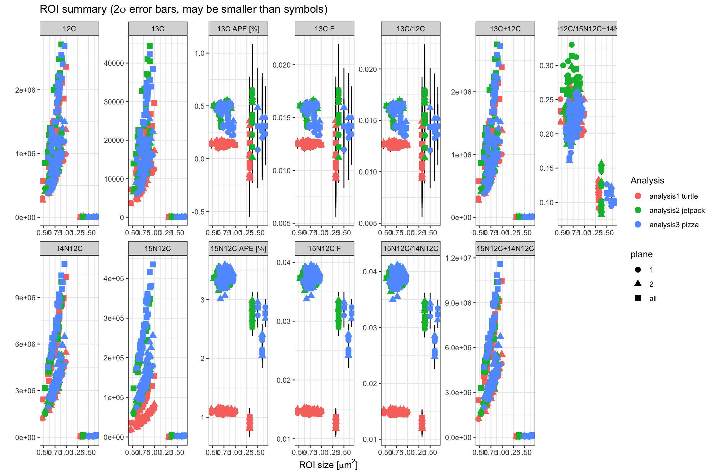

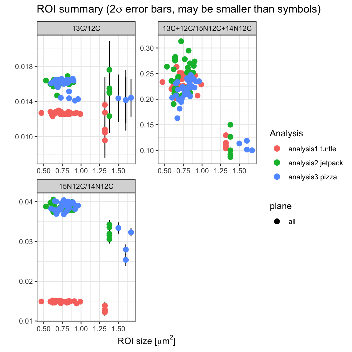
Focus in on the combined counts (not the individual planes from the z-stack) and look just at ratios:

last_plot() %+% (data %>% filter(plane == "all", data_type == "ratio"))

Ion maps

Again, loading the ion maps for all 3 analyses.

maps <- 
  load_LANS_maps (
    analysis = c("analysis1", "analysis2", "analysis3"),
    base_dir = folder
  )

## INFO: folder 'analysis1' read successfully.
##       Ion map data for 256 x 256 pixel frame (10.014 microm^2) for 4 ions recovered: 12C, 13C, 14N12C, 15N12C.
##       37 ROIs identified in the frame.

## INFO: folder 'analysis2' read successfully.
##       Ion map data for 256 x 256 pixel frame (10.014 microm^2) for 4 ions recovered: 12C, 13C, 14N12C, 15N12C.
##       33 ROIs identified in the frame.

## INFO: folder 'analysis3' read successfully.
##       Ion map data for 256 x 256 pixel frame (10.014 microm^2) for 4 ions recovered: 12C, 13C, 14N12C, 15N12C.
##       34 ROIs identified in the frame.

The data in these looks similar to the summary data frame except that it is broken out pixel by pixel:

maps %>% head(n=10) %>% kable()

analysis	x.px	y.px	frame_size.px	x.um	y.um	frame_size.um	variable	data_type	value	sigma
analysis1	1	1	256	0.0391172	0.0391172	10.014	12C	ion_count	1721	41.48494
analysis1	1	2	256	0.0391172	0.0782344	10.014	12C	ion_count	1694	41.15823
analysis1	1	3	256	0.0391172	0.1173516	10.014	12C	ion_count	1508	38.83298
analysis1	1	4	256	0.0391172	0.1564688	10.014	12C	ion_count	1297	36.01389
analysis1	1	5	256	0.0391172	0.1955859	10.014	12C	ion_count	1136	33.70460
analysis1	1	6	256	0.0391172	0.2347031	10.014	12C	ion_count	786	28.03569
analysis1	1	7	256	0.0391172	0.2738203	10.014	12C	ion_count	702	26.49528
analysis1	1	8	256	0.0391172	0.3129375	10.014	12C	ion_count	453	21.28380
analysis1	1	9	256	0.0391172	0.3520547	10.014	12C	ion_count	319	17.86057
analysis1	1	10	256	0.0391172	0.3911719	10.014	12C	ion_count	220	14.83240

To make it easier to plot these kind of maps, lans2r provides a convenience functoin plot_maps but of course this could be adjusted as needed (look at the source code to see how this one is made). By default ion counts are normalized for each ion so they can be visualized on the same scale.

plot_maps(maps)

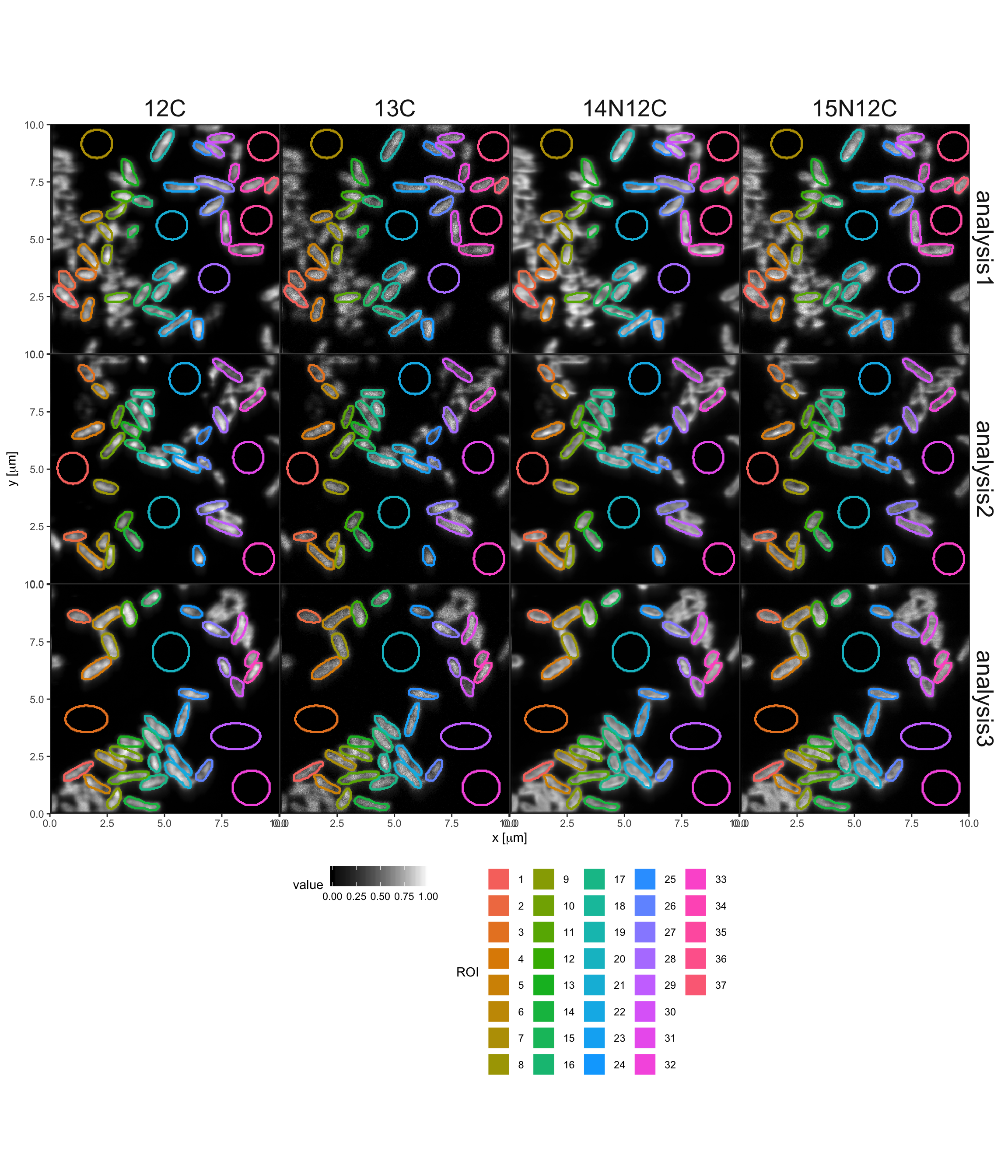
Focusing in on just one ion, we can ditch the normalization, and let’s also not draw ROIs for a direct look. Also, because it’s a ggplot, all ggplot modifications of the plot are fair game.

plot_maps(maps %>% filter(variable == "14N12C", analysis %in% c("analysis1", "analysis2")), 
          normalize = FALSE, draw_ROIs = FALSE) + 
  theme(legend.position = "right") + labs(fill = "ion count")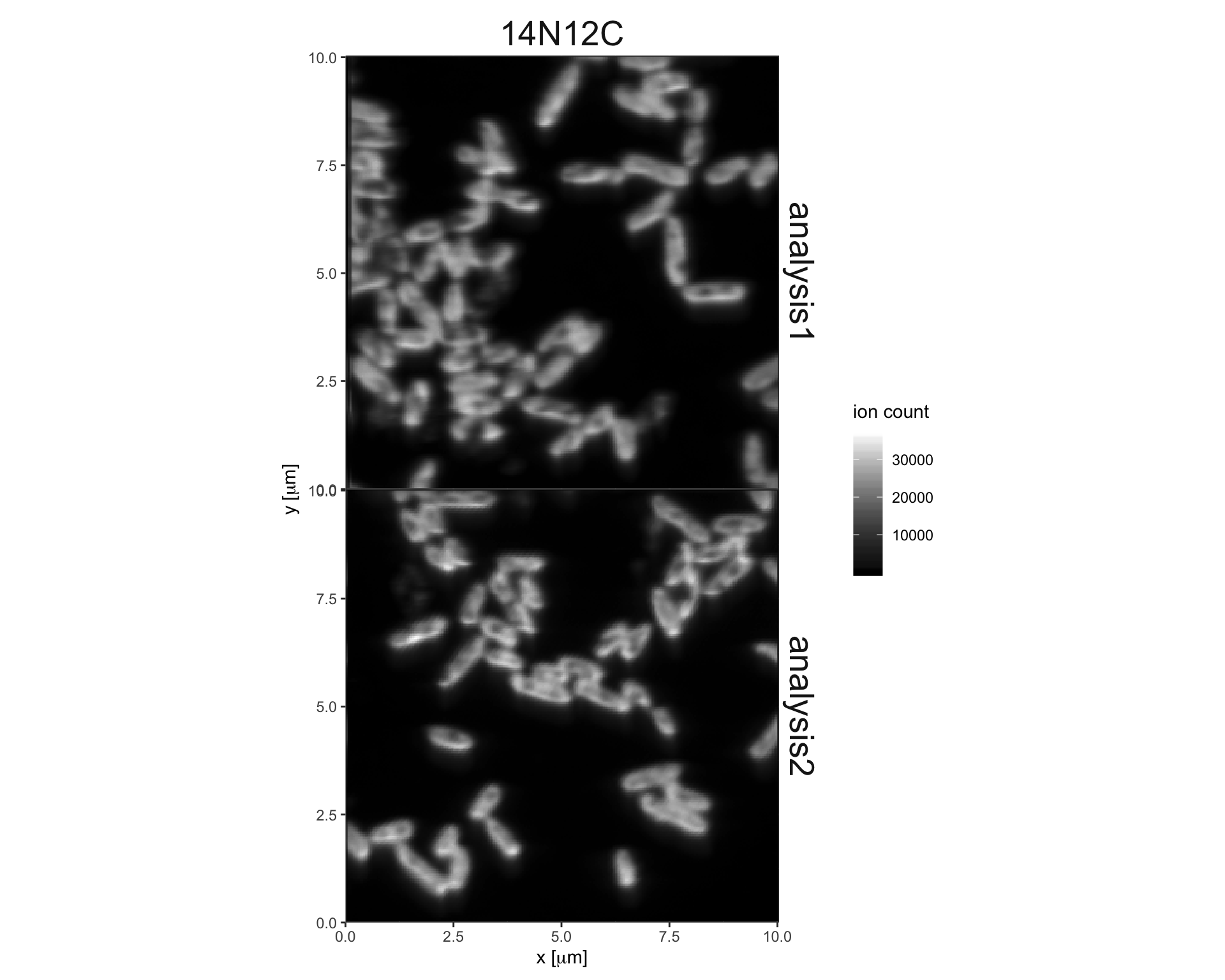

Future directions

Note that for plotting maps, lans2r does not (yet) support any smoothing so although the plot_maps function theoretically supports plotting ratios and abundances as well (which can be calculated from the maps data the same way using calculate_ratios and calculate_abundances), in practice this does not work so well because individual pixels often have extreme values offsetting proper scaling. This might be part of future expansions if the package sees a lot of use so please email with suggestions if you find it helpful.

Load data

ROI overview data

Overview

Plotting

Ion maps

Future directions

Contents